

How To Draw Graph In Latex
LaTeX options for graphs
This module provides a class to hold, dispense and employ various options for rendering a graph in LaTeX, in addition to providing the code that actually generates a LaTeX representation of a (combinatorial) graph.
AUTHORS:
-
Rob Beezer (2009-05-20):
GraphLatexgrade -
Fidel Barerra Cruz (2009-05-xx):
tkz-graphcommands to return a graph -
Nicolas One thousand. Thiéry (2010-02): dot2tex/graphviz interface
-
Rob Beezer (2010-05-29): Extended range of
tkz-graphoptions
LaTeX Versions of Graphs
Many mathematical objects in Sage take LaTeX representations, and graphs are no exception. For a graph g , the command view(g) , issued at the Sage command line or in the notebook, volition create a graphic version of one thousand . Similarly, latex(g) volition return a (long) string that is a representation of the graph in LaTeX. Other ways of employing LaTeX in Sage, such as %latex in a notebook cell, or the Typeset checkbox in the notebook, will handle g appropriately.
Support through the tkz-graph package is by Alain Matthes, the author of tkz-graph , whose piece of work can be constitute at https://www.ctan.org/pkg/tkz-graph.
The range of possible options for customizing the advent of a graph are carefully documented at sage.graphs.graph_latex.GraphLatex.set_option() . Equally a broad overview, the post-obit options are supported:
-
Pre-built Styles: the pre-built styles of the tkz-graph package provide nice drawings quickly
-
Dimensions: tin be specified in natural units, then uniformly scaled after blueprint piece of work
-
Vertex Colors: the perimeter and fill color for vertices can be specified, including on a per-vertex basis
-
Vertex Shapes: may be circles, shaded spheres, rectangles or diamonds, including on a per-vertex basis
-
Vertex Sizes: may be specified as minimums, and will automatically sized to contain vertex labels, including on a per-vertex footing
-
Vertex Labels: tin use latex formatting, and may have their colors specified, including on a per-vertex basis
-
Vertex Label Placement: can be interior to the vertex, or external at a configurable location
-
Edge Colors: a solid color with or without a second color down the eye, on a per-edge basis
-
Edge Thickness: can exist set, including on a per-border ground
-
Edge Labels: can apply latex formatting, and may accept their colors specified, including on a per-border footing
-
Edge Label Placement: can be to the left, right, above, below, inline, and then sloped or horizontal
-
Digraph Edges: are slightly curved, with arrowheads
-
Loops: may be specified by their size, and with a direction equaling one of the four compass points
To utilise LaTeX in Sage you of form need a working TeX installation and it will piece of work all-time if you have the dvipng and catechumen utilities. For graphs you need the tkz-graph.sty and tkz-berge.sty fashion files of the tkz-graph package. TeX, dvipng, and convert should exist widely available through parcel managers or installers. Y'all may demand to install the tkz-graph style files in the appropriate locations, a chore beyond the telescopic of this introduction. Primary locations for these programs are:
-
TeX: http://ctan.org/
-
dvipng: http://sourceforge.net/projects/dvipng/
-
convert: http://www.imagemagick.org (the ImageMagick suite)
-
tkz-graph: https://www.ctan.org/pkg/tkz-graph
Customizing the output is achieved in several ways. Suppose g is a graph, then chiliad.set_latex_options() can be used to efficiently set or alter diverse options. Setting private options, or querying options, can be accomplished by first using a command like opts = g.latex_options() to obtain a sage.graphs.graph_latex.GraphLatex object which has several methods to ready and recall options.
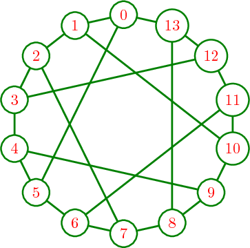
Here is a minimal session demonstrating how to use these features. The following setup should work in the notebook or at the command-line.:
sage: H = graphs . HeawoodGraph () sage: H . set_latex_options ( ....: graphic_size = ( 5 , 5 ), ....: vertex_size = 0.2 , ....: edge_thickness = 0.04 , ....: edge_color = 'green' , ....: vertex_color = 'light-green' , ....: vertex_label_color = 'carmine' ....: ) At this betoken, view(H) should phone call pdflatex to procedure the string created by latex(H) and and then brandish the resulting graphic.
To employ this prototype in a LaTeX document, you could of class just re-create and save the resulting graphic. However, the latex() control will produce the underlying LaTeX code, which tin can exist incorporated into a standalone LaTeX document.:
sage: from sage.graphs.graph_latex import check_tkz_graph sage: check_tkz_graph () # random - depends on TeX installation sage: latex ( H ) \brainstorm{tikzpicture} \definecolor{cv0}{rgb}{0.0,0.502,0.0} \definecolor{cfv0}{rgb}{one.0,1.0,1.0} \definecolor{clv0}{rgb}{i.0,0.0,0.0} \definecolor{cv1}{rgb}{0.0,0.502,0.0} \definecolor{cfv1}{rgb}{1.0,1.0,1.0} \definecolor{clv1}{rgb}{1.0,0.0,0.0} \definecolor{cv2}{rgb}{0.0,0.502,0.0} \definecolor{cfv2}{rgb}{1.0,one.0,i.0} \definecolor{clv2}{rgb}{one.0,0.0,0.0} \definecolor{cv3}{rgb}{0.0,0.502,0.0} \definecolor{cfv3}{rgb}{1.0,i.0,1.0} \definecolor{clv3}{rgb}{1.0,0.0,0.0} \definecolor{cv4}{rgb}{0.0,0.502,0.0} \definecolor{cfv4}{rgb}{1.0,ane.0,1.0} \definecolor{clv4}{rgb}{1.0,0.0,0.0} \definecolor{cv5}{rgb}{0.0,0.502,0.0} \definecolor{cfv5}{rgb}{1.0,1.0,1.0} \definecolor{clv5}{rgb}{ane.0,0.0,0.0} \definecolor{cv6}{rgb}{0.0,0.502,0.0} \definecolor{cfv6}{rgb}{1.0,ane.0,1.0} \definecolor{clv6}{rgb}{one.0,0.0,0.0} \definecolor{cv7}{rgb}{0.0,0.502,0.0} \definecolor{cfv7}{rgb}{1.0,ane.0,1.0} \definecolor{clv7}{rgb}{1.0,0.0,0.0} \definecolor{cv8}{rgb}{0.0,0.502,0.0} \definecolor{cfv8}{rgb}{1.0,i.0,i.0} \definecolor{clv8}{rgb}{1.0,0.0,0.0} \definecolor{cv9}{rgb}{0.0,0.502,0.0} \definecolor{cfv9}{rgb}{1.0,1.0,1.0} \definecolor{clv9}{rgb}{1.0,0.0,0.0} \definecolor{cv10}{rgb}{0.0,0.502,0.0} \definecolor{cfv10}{rgb}{1.0,ane.0,one.0} \definecolor{clv10}{rgb}{1.0,0.0,0.0} \definecolor{cv11}{rgb}{0.0,0.502,0.0} \definecolor{cfv11}{rgb}{i.0,i.0,1.0} \definecolor{clv11}{rgb}{ane.0,0.0,0.0} \definecolor{cv12}{rgb}{0.0,0.502,0.0} \definecolor{cfv12}{rgb}{i.0,1.0,i.0} \definecolor{clv12}{rgb}{1.0,0.0,0.0} \definecolor{cv13}{rgb}{0.0,0.502,0.0} \definecolor{cfv13}{rgb}{1.0,1.0,1.0} \definecolor{clv13}{rgb}{one.0,0.0,0.0} \definecolor{cv0v1}{rgb}{0.0,0.502,0.0} \definecolor{cv0v5}{rgb}{0.0,0.502,0.0} \definecolor{cv0v13}{rgb}{0.0,0.502,0.0} \definecolor{cv1v2}{rgb}{0.0,0.502,0.0} \definecolor{cv1v10}{rgb}{0.0,0.502,0.0} \definecolor{cv2v3}{rgb}{0.0,0.502,0.0} \definecolor{cv2v7}{rgb}{0.0,0.502,0.0} \definecolor{cv3v4}{rgb}{0.0,0.502,0.0} \definecolor{cv3v12}{rgb}{0.0,0.502,0.0} \definecolor{cv4v5}{rgb}{0.0,0.502,0.0} \definecolor{cv4v9}{rgb}{0.0,0.502,0.0} \definecolor{cv5v6}{rgb}{0.0,0.502,0.0} \definecolor{cv6v7}{rgb}{0.0,0.502,0.0} \definecolor{cv6v11}{rgb}{0.0,0.502,0.0} \definecolor{cv7v8}{rgb}{0.0,0.502,0.0} \definecolor{cv8v9}{rgb}{0.0,0.502,0.0} \definecolor{cv8v13}{rgb}{0.0,0.502,0.0} \definecolor{cv9v10}{rgb}{0.0,0.502,0.0} \definecolor{cv10v11}{rgb}{0.0,0.502,0.0} \definecolor{cv11v12}{rgb}{0.0,0.502,0.0} \definecolor{cv12v13}{rgb}{0.0,0.502,0.0} % \Vertex[fashion={minimum size=0.2cm,depict=cv0,fill=cfv0,text=clv0,shape=circumvolve},LabelOut=simulated,50=\hbox{$0$},x=2.5cm,y=5.0cm]{v0} \Vertex[style={minimum size=0.2cm,draw=cv1,make full=cfv1,text=clv1,shape=circle},LabelOut=false,L=\hbox{$1$},ten=1.3874cm,y=iv.7524cm]{v1} \Vertex[style={minimum size=0.2cm,describe=cv2,fill up=cfv2,text=clv2,shape=circumvolve},LabelOut=imitation,50=\hbox{$two$},x=0.4952cm,y=4.0587cm]{v2} \Vertex[style={minimum size=0.2cm,draw=cv3,fill=cfv3,text=clv3,shape=circle},LabelOut=false,L=\hbox{$3$},10=0.0cm,y=3.0563cm]{v3} \Vertex[manner={minimum size=0.2cm,draw=cv4,make full=cfv4,text=clv4,shape=circle},LabelOut=false,L=\hbox{$iv$},x=0.0cm,y=1.9437cm]{v4} \Vertex[style={minimum size=0.2cm,describe=cv5,fill up=cfv5,text=clv5,shape=circle},LabelOut=simulated,50=\hbox{$v$},10=0.4952cm,y=0.9413cm]{v5} \Vertex[way={minimum size=0.2cm,draw=cv6,fill=cfv6,text=clv6,shape=circumvolve},LabelOut=imitation,L=\hbox{$vi$},x=1.3874cm,y=0.2476cm]{v6} \Vertex[manner={minimum size=0.2cm,draw=cv7,fill up=cfv7,text=clv7,shape=circle},LabelOut=false,L=\hbox{$7$},10=2.5cm,y=0.0cm]{v7} \Vertex[way={minimum size=0.2cm,draw=cv8,fill up=cfv8,text=clv8,shape=circle},LabelOut=fake,Fifty=\hbox{$eight$},10=iii.6126cm,y=0.2476cm]{v8} \Vertex[style={minimum size=0.2cm,draw=cv9,fill=cfv9,text=clv9,shape=circle},LabelOut=simulated,L=\hbox{$nine$},ten=4.5048cm,y=0.9413cm]{v9} \Vertex[style={minimum size=0.2cm,depict=cv10,fill=cfv10,text=clv10,shape=circle},LabelOut=faux,L=\hbox{$10$},10=5.0cm,y=1.9437cm]{v10} \Vertex[style={minimum size=0.2cm,draw=cv11,fill=cfv11,text=clv11,shape=circumvolve},LabelOut=false,L=\hbox{$11$},10=5.0cm,y=3.0563cm]{v11} \Vertex[fashion={minimum size=0.2cm,draw=cv12,fill=cfv12,text=clv12,shape=circle},LabelOut=imitation,L=\hbox{$12$},ten=four.5048cm,y=4.0587cm]{v12} \Vertex[style={minimum size=0.2cm,describe=cv13,fill=cfv13,text=clv13,shape=circle},LabelOut=fake,L=\hbox{$13$},ten=3.6126cm,y=4.7524cm]{v13} % \Edge[lw=0.04cm,fashion={colour=cv0v1,},](v0)(v1) \Edge[lw=0.04cm,style={color=cv0v5,},](v0)(v5) \Edge[lw=0.04cm,way={colour=cv0v13,},](v0)(v13) \Edge[lw=0.04cm,style={color=cv1v2,},](v1)(v2) \Edge[lw=0.04cm,way={color=cv1v10,},](v1)(v10) \Edge[lw=0.04cm,style={color=cv2v3,},](v2)(v3) \Border[lw=0.04cm,style={color=cv2v7,},](v2)(v7) \Edge[lw=0.04cm,style={colour=cv3v4,},](v3)(v4) \Edge[lw=0.04cm,way={color=cv3v12,},](v3)(v12) \Edge[lw=0.04cm,style={color=cv4v5,},](v4)(v5) \Edge[lw=0.04cm,style={color=cv4v9,},](v4)(v9) \Edge[lw=0.04cm,style={colour=cv5v6,},](v5)(v6) \Edge[lw=0.04cm,style={color=cv6v7,},](v6)(v7) \Edge[lw=0.04cm,mode={color=cv6v11,},](v6)(v11) \Edge[lw=0.04cm,style={colour=cv7v8,},](v7)(v8) \Edge[lw=0.04cm,style={color=cv8v9,},](v8)(v9) \Edge[lw=0.04cm,way={colour=cv8v13,},](v8)(v13) \Edge[lw=0.04cm,way={color=cv9v10,},](v9)(v10) \Border[lw=0.04cm,mode={color=cv10v11,},](v10)(v11) \Border[lw=0.04cm,style={color=cv11v12,},](v11)(v12) \Edge[lw=0.04cm,style={color=cv12v13,},](v12)(v13) % \end{tikzpicture} EXAMPLES:
This instance illustrates switching betwixt the congenital-in styles when using the tkz_graph format.:
sage: g = graphs . PetersenGraph () sage: k . set_latex_options ( tkz_style = 'Classic' ) sage: from sage.graphs.graph_latex import check_tkz_graph sage: check_tkz_graph () # random - depends on TeX installation sage: latex ( g ) \brainstorm{tikzpicture} \GraphInit[vstyle=Classic] ... \end{tikzpicture} sage: opts = g . latex_options () sage: opts LaTeX options for Petersen graph: {'tkz_style': 'Classic'} sage: thou . set_latex_options ( tkz_style = 'Art' ) sage: opts . get_option ( 'tkz_style' ) 'Fine art' sage: opts LaTeX options for Petersen graph: {'tkz_style': 'Fine art'} sage: latex ( g ) \brainstorm{tikzpicture} \GraphInit[vstyle=Art] ... \end{tikzpicture} This example illustrates using the optional dot2tex module:
sage: g = graphs . PetersenGraph () sage: grand . set_latex_options ( format = 'dot2tex' , prog = 'neato' ) sage: from sage.graphs.graph_latex import check_tkz_graph sage: check_tkz_graph () # random - depends on TeX installation sage: latex ( grand ) # optional - dot2tex graphviz \brainstorm{tikzpicture}[>=latex,line bring together=bevel,] ... \end{tikzpicture} Amid other things, this supports the flexible edge_options option (run into sage.graphs.generic_graph.GenericGraph.graphviz_string() ); here nosotros color in red all edges touching the vertex 0 :
sage: one thousand = graphs . PetersenGraph () sage: g . set_latex_options ( format = "dot2tex" , edge_options = lambda u_v_label : { "color" : "scarlet" } if u_v_label [ 0 ] == 0 else {}) sage: latex ( thousand ) # optional - dot2tex graphviz \begin{tikzpicture}[>=latex,line join=bevel,] ... \terminate{tikzpicture} GraphLatex grade and functions
- form sage.graphs.graph_latex. GraphLatex ( graph , ** options )
-
Bases:
sage.structure.sage_object.SageObjectA class to concur, manipulate and employ options for converting a graph to LaTeX.
This class serves two purposes. First information technology holds the values of diverse options designed to piece of work with the
tkz-graphLaTeX package for rendering graphs. As such, a graph that uses this form will concur a reference to it. 2d, this form contains the code to convert a graph into the corresponding LaTeX constructs, returning a string.EXAMPLES:
sage: from sage.graphs.graph_latex import GraphLatex sage: opts = GraphLatex ( graphs . PetersenGraph ()) sage: opts LaTeX options for Petersen graph: {} sage: g = graphs . PetersenGraph () sage: opts = k . latex_options () sage: 1000 == loads ( dumps ( g )) True
- dot2tex_picture ( )
-
Call
dot2texto construct a string of LaTeX commands representing a graph as atikzpicture.EXAMPLES:
sage: g = digraphs . ButterflyGraph ( i ) sage: from sage.graphs.graph_latex import check_tkz_graph sage: check_tkz_graph () # random - depends on TeX installation sage: print ( grand . latex_options () . dot2tex_picture ()) # optional - dot2tex graphviz \begin{tikzpicture}[>=latex,line join=bevel,] %% \node (node_...) at (...bp,...bp) [draw,draw=none] {$\left(...\correct)$}; \node (node_...) at (...bp,...bp) [describe,draw=none] {$\left(...\right)$}; \node (node_...) at (...bp,...bp) [draw,draw=none] {$\left(...\correct)$}; \node (node_...) at (...bp,...bp) [draw,describe=none] {$\left(...\right)$}; \depict [blackness,->] (node_...) ..controls (...bp,...bp) and (...bp,...bp) .. (node_...); \describe [blackness,->] (node_...) ..controls (...bp,...bp) and (...bp,...bp) .. (node_...); \draw [black,->] (node_...) ..controls (...bp,...bp) and (...bp,...bp) .. (node_...); \draw [black,->] (node_...) ..controls (...bp,...bp) and (...bp,...bp) .. (node_...); % \stop{tikzpicture}
We make sure trac ticket #13624 is stock-still:
sage: G = DiGraph () sage: Thousand . add_edge ( 3333 , 88 , 'my_label' ) sage: G . set_latex_options ( edge_labels = Truthful ) sage: impress ( One thousand . latex_options () . dot2tex_picture ()) # optional - dot2tex graphviz \begin{tikzpicture}[>=latex,line join=bevel,] %% \node (node_...) at (...bp,...bp) [draw,draw=none] {$...$}; \node (node_...) at (...bp,...bp) [draw,draw=none] {$...$}; \draw [black,->] (node_...) ..controls (...bp,...bp) and (...bp,...bp) .. (node_...); \definecolor{strokecol}{rgb}{0.0,0.0,0.0}; \pgfsetstrokecolor{strokecol} \draw (...bp,...bp) node {$\text{\texttt{my{\char`\_}label}}$}; % \stop{tikzpicture}
Check that trac ticket #25120 is stock-still:
sage: Chiliad = Graph ([( 0 , 1 )]) sage: One thousand . set_latex_options ( edge_colors = {( 0 , one ): 'ruddy' }) sage: print ( G . latex_options () . dot2tex_picture ()) # optional - dot2tex graphviz \begin{tikzpicture}[>=latex,line join=bevel,] ... \draw [red,] (node_0) ... (node_1); ... \end{tikzpicture}
Note
There is a lot of overlap between what
tkz_pictureanddot2texdo. It would be best to merge them!dot2texprobably can work withoutgraphvizif layout information is provided.
- get_option ( option_name )
-
Render the current value of the named option.
INPUT:
-
option_name– the name of an choice
OUTPUT:
If the name is non present in
__graphlatex_optionsit is an fault to ask for information technology. If an option has not been fix then the default value is returned. Otherwise, the value of the option is returned.EXAMPLES:
sage: thousand = graphs . PetersenGraph () sage: opts = thou . latex_options () sage: opts . set_option ( 'tkz_style' , 'Art' ) sage: opts . get_option ( 'tkz_style' ) 'Art' sage: opts . set_option ( 'tkz_style' ) sage: opts . get_option ( 'tkz_style' ) == "Custom" True sage: opts . get_option ( 'bad_name' ) Traceback (most recent phone call last): ... ValueError: bad_name is not a Latex option for a graph.
-
- latex ( )
-
Return a string in LaTeX representing a graph.
This is the command that is invoked by
sage.graphs.generic_graph.GenericGraph._latex_for a graph, so it returns a cord of LaTeX commands that can be incorporated into a LaTeX document unmodified. The exact contents of this cord are influenced by the options set via the methodssage.graphs.generic_graph.GenericGraph.set_latex_options(),set_option(), andset_options().By setting the
formatoption different packages can be used to create the latex version of a graph. Supported packages aretkz-graphanddot2tex.EXAMPLES:
sage: from sage.graphs.graph_latex import check_tkz_graph sage: check_tkz_graph () # random - depends on TeX installation sage: grand = graphs . CompleteGraph ( 2 ) sage: opts = g . latex_options () sage: impress ( opts . latex ()) \begin{tikzpicture} \definecolor{cv0}{rgb}{0.0,0.0,0.0} \definecolor{cfv0}{rgb}{1.0,1.0,1.0} \definecolor{clv0}{rgb}{0.0,0.0,0.0} \definecolor{cv1}{rgb}{0.0,0.0,0.0} \definecolor{cfv1}{rgb}{1.0,1.0,i.0} \definecolor{clv1}{rgb}{0.0,0.0,0.0} \definecolor{cv0v1}{rgb}{0.0,0.0,0.0} % \Vertex[mode={minimum size=one.0cm,draw=cv0,fill=cfv0,text=clv0,shape=circle},LabelOut=simulated,50=\hbox{$0$},10=2.5cm,y=5.0cm]{v0} \Vertex[way={minimum size=i.0cm,describe=cv1,fill up=cfv1,text=clv1,shape=circle},LabelOut=fake,L=\hbox{$1$},x=2.5cm,y=0.0cm]{v1} % \Edge[lw=0.1cm,style={colour=cv0v1,},](v0)(v1) % \finish{tikzpicture}
We check that trac ticket #22070 is fixed:
sage: edges = [( i ,( i + 1 ) % 3,a) for i,a in enumerate('abc')] sage: G_with_labels = DiGraph ( edges ) sage: C = [[ 0 , 1 ], [ 2 ]] sage: kwds = dict ( subgraph_clusters = C , color_by_label = True , prog = 'dot' , format = 'dot2tex' ) sage: opts = G_with_labels . latex_options () sage: opts . set_options ( edge_labels = True , ** kwds ) # optional - dot2tex graphviz sage: latex ( G_with_labels ) # optional - dot2tex graphviz \begin{tikzpicture}[>=latex,line join=bevel,] %% \begin{scope} \pgfsetstrokecolor{black} \definecolor{strokecol}{rgb}{...}; \pgfsetstrokecolor{strokecol} \definecolor{fillcol}{rgb}{...}; \pgfsetfillcolor{fillcol} \filldraw ... cycle; \end{telescopic} \begin{scope} \pgfsetstrokecolor{black} \definecolor{strokecol}{rgb}{...}; \pgfsetstrokecolor{strokecol} \definecolor{fillcol}{rgb}{...}; \pgfsetfillcolor{fillcol} \filldraw ... cycle; \end{scope} ... \cease{tikzpicture}
- set_option ( option_name , option_value = None )
-
Ready, change, clear a LaTeX selection for controlling the rendering of a graph.
The possible options are documented hither, because ultimately it is this routine that sets the values. However, the
sage.graphs.generic_graph.GenericGraph.set_latex_options()method is the easiest way to prepare options, and allows several to be set at once.INPUT:
-
option_name– a cord for a latex option contained in the listsage.graphs.graph_latex.GraphLatex.__graphlatex_options. AValueErroris raised if the pick is not allowed. -
option_value– a value for the option. If omitted, or set toNone, the pick will utilise the default value.
The output tin can be either handled internally past
Sage, or delegated to the external softwaredot2texandgraphviz. This is controlled by the optionformat:-
format– cord (default:'tkz_graph'); either'dot2tex'or'tkz_graph'.
If format is
'dot2tex', then all the LaTeX generation volition be delegated todot2tex(which must exist installed).For
tkz_graph, the possible option names, and associated values are given below. This offset group allows you to set a fashion for a graph and specify some sizes related to the eventual epitome. (For more information consult the documentation for thetkz-graphpackage.)-
tkz_style– string (default:'Custom'); the name of a pre-definedtkz-graphmode such as'Shade','Art','Normal','Dijkstra','Welsh','Archetype', and'Elementary', or the cord'Custom'. Using one of these styles alone volition often give a reasonably good drawing with minimal effort. For a custom advent ready this to'Custom'and apply the options described below to override the default values. -
units– string (default:'cm') – a natural unit of measurement used for all dimensions. Possible values are:'in','mm','cm','pt','em','ex'. -
calibration– bladder (default:i.0); a dimensionless number that multiplies every linear dimension. So you tin can design at sizes yous are accustomed to, then shrink or expand to meet other needs. Though fonts practise not calibration. -
graphic_size– tuple (default:(5, 5)); overall dimensions (width, length) of the bounding box around the unabridged graphic image. -
margins– 4-tuple (default:(0, 0, 0, 0)); portion of graphic given over to a plain border equally a tuple of four numbers: (left, right, top, lesser). These are subtracted from thegraphic_sizeto create the expanse left for the vertices of the graph itself. Annotation that the processing washed by Sage will trim the graphic downward to the minimum possible size, removing any border. So this is only useful if yous use the latex string in a latex document.
If not using a pre-built manner the following options are used, and then the post-obit defaults will apply. It is non possible to begin with a pre-built style and modify it (other than editing the latex string past mitt after the fact).
-
vertex_color– (default:'blackness'); a single color to use as the default for outline of vertices. For thesphereshape this color is used for the entire vertex, which is drawn with a 3D shading. Colors must be specified as a string recognized by the matplotlib library: a standard color proper noun similar'ruby', or a hex string like'#2D87A7', or a single character from the choices'rgbcmykw'. Additionally, a number between 0 and 1 will create a grayscale value. These colour specifications are consistent throughout the options for atikzpicture. -
vertex_colors– a lexicon whose keys are vertices of the graph and whose values are colors. These will be used to color the outline of vertices. See the explanation to a higher place for thevertex_coloroption to encounter possible values. These values demand only be specified for a proper subset of the vertices. Specified values volition supersede a default value. -
vertex_fill_color– (default:'white'); a single colour to apply equally the default for the fill color of vertices. Run across the explanation higher up for thevertex_coloroption to see possible values. This color is ignored for thespherevertex shape. -
vertex_fill_colors– a dictionary whose keys are vertices of the graph and whose values are colors. These will exist used to fill the interior of vertices. See the explanation above for thevertex_coloroption to run into possible values. These values demand only be specified for a proper subset of the vertices. Specified values will supplant a default value. -
vertex_shape– string (default:'circle'); specifies the shape of the vertices. Allowable values are'circumvolve','sphere','rectangle','diamond'. The sphere shape has a 3D look to its coloring and is uses but i color, that specified byvertex_colorandvertex_colors, which are usually used for the outline of the vertex. -
vertex_shapes– a dictionary whose keys are vertices of the graph and whose values are shapes. Run intovertex_shapefor the commanded possibilities. -
vertex_size– bladder (default: 1.0); the minimum size of a vertex every bit a number. Vertices will aggrandize to contain their labels if the labels are placed within the vertices. If you set this value to null the vertex will be equally small as possible (up to tkz-graph'southward "inner sep" parameter), while nonetheless containing labels. Even so, if labels are not of a uniform size, then the vertices volition non be either. -
vertex_sizes– a dictionary of sizes for some of the vertices. -
vertex_labels– boolean (default:True); determine whether or not to display the vertex labels. IfFakesubsequent options about vertex labels are ignored. -
vertex_labels_math– boolean (default:Truthful); whenTrue, if a characterization is a string that begins and ends with dollar signs, so the string will be rendered as a latex string. Otherwise, the characterization volition be automatically subjected to thelatex()method and rendered appropriately. IfFalsethe label is rendered equally its textual representation co-ordinate to the_reprmethod. Support for arbitrarily-complicated mathematics is not specially robust. -
vertex_label_color– (default:'black'); a single color to employ as the default for labels of vertices. See the explanation above for thevertex_coloroption to run across possible values. -
vertex_label_colors– a dictionary whose keys are vertices of the graph and whose values are colors. These will be used for the text of the labels of vertices. See the caption higher up for thevertex_coloroption to see possible values. These values need only be specified for a proper subset of the vertices. Specified values will supersede a default value. -
vertex_label_placement– (default:'center'); if'centre'the label is centered in the interior of the vertex and the vertex will expand to contain the label. Giving instead a pair of numbers will place the label exterior to the vertex at a certain distance from the edge, and at an bending to the positive ten-centrality, similar in spirit to polar coordinates. -
vertex_label_placements– a dictionary of placements indexed by the vertices. See the explanation forvertex_label_placementfor the possible values. -
edge_color– (default:'black'); a single color to utilize as the default for an edge. See the explanation in a higher place for thevertex_colorselection to run into possible values. -
edge_colors– a lexicon whose keys are edges of the graph and whose values are colors. These will exist used to color the edges. See the explanation in a higher place for thevertex_colorpick to meet possible values. These values demand only be specified for a proper subset of the vertices. Specified values will replace a default value. -
edge_fills– boolean (default:Simulated); whether an edge has a 2d color running downwardly the middle. This can be a useful effect for highlighting edge crossings. -
edge_fill_color– (default:'blackness'); a single color to use as the default for the fill color of an edge. The boolean switchedge_fillsmust be gear up to True for this to take an effect. See the explanation above for thevertex_coloroption to run into possible values. -
edge_fill_colors– a dictionary whose keys are edges of the graph and whose values are colors. Meet the explanation to a higher place for thevertex_coloroption to encounter possible values. These values need only be specified for a proper subset of the vertices. Specified values volition supersede a default value. -
edge_thickness– float (default: 0.one); specifies the width of the edges. Annotation thattkz-graphdoes non interpret this number for loops. -
edge_thicknesses– a dictionary of thicknesses for some of the edges of a graph. These values need only exist specified for a proper subset of the vertices. Specified values volition supervene upon a default value. -
edge_labels– boolean (default:Imitation); determine if edge labels are shown. IfFalsesubsequent options about edge labels are ignored. -
edge_labels_math– boolean (default:True); control how edge labels are rendered. Read the caption for thevertex_labels_mathoption, which behaves identically. Support for arbitrarily-complicated mathematics is not especially robust. -
edge_label_color– (default:'black'); a single colour to use every bit the default for labels of edges. Run into the explanation higher up for thevertex_colorpick to see possible values. -
edge_label_colors– a dictionary whose keys are edges of the graph and whose values are colors. These will exist used for the text of the labels of edges. See the explanation above for thevertex_colorchoice to see possible values. These values demand only be specified for a proper subset of the vertices. Specified values volition supersede a default value. Note that labels must be used for this to have any effect, and no care is taken to ensure that label and fill up colors piece of work well together. -
edge_label_sloped– boolean (default:True); specifies how edge labels are identify.Fauxresults in a horizontal label, whileTrueways the label is rotated to follow the management of the edge information technology labels. -
edge_label_slopes– a dictionary of booleans, indexed by some subset of the edges. Encounter theedge_label_slopedoption for a description of sloped edge labels. -
edge_label_placement– (default: 0.50); either a number betwixt 0.0 and 1.0, or i of:'above','below','left','correct'. These conform the location of an edge label along an edge. A number specifies how far along the edge the label is located.'left'and'right'are conveniences.'to a higher place'and'below'move the label off the border itself while leaving information technology almost the midpoint of the edge. The default value of0.50places the label on the midpoint of the edge. -
edge_label_placements– a dictionary of border placements, indexed past the edges. Come across theedge_label_placementoption for a description of the allowable values. -
loop_placement– (default:(3.0, 'NO')); determine how loops are rendered. the first element of the pair is a distance, which determines how large the loop is and the second element is a string specifying a compass betoken (North, South, Eastward, Westward) equally one of'NO','SO','EA','WE'. -
loop_placements– a dictionary of loop placements. See theloop_placementsoption for the allowable values. While loops are technically edges, this dictionary is indexed by vertices.
For the
'dot2tex'format, the possible choice names and associated values are given below:-
prog– string; the plan used for the layout. It must be a string respective to one of the software of the graphviz suite:'dot','neato','twopi','circo'or'fdp'. -
edge_labels– boolean (default:False); whether to display the labels on edges. -
edge_colors– a color; tin exist used to set a global colour to the edge of the graph. -
color_by_label– boolean (default:False); colors the edges co-ordinate to their labels -
subgraph_clusters– (default:[]) a list of lists of vertices, if supported by the layout engine, nodes belonging to the same cluster subgraph are drawn together, with the entire drawing of the cluster contained within a bounding rectangle.
OUTPUT:
There are none. Success happens silently.
EXAMPLES:
Set, then modify, so articulate the
tkz_styleselection, and finally show an error for an unrecognized option proper name:sage: one thousand = graphs . PetersenGraph () sage: opts = g . latex_options () sage: opts LaTeX options for Petersen graph: {} sage: opts . set_option ( 'tkz_style' , 'Art' ) sage: opts LaTeX options for Petersen graph: {'tkz_style': 'Fine art'} sage: opts . set_option ( 'tkz_style' , 'Elementary' ) sage: opts LaTeX options for Petersen graph: {'tkz_style': 'Simple'} sage: opts . set_option ( 'tkz_style' ) sage: opts LaTeX options for Petersen graph: {} sage: opts . set_option ( 'bad_name' , 'nonsense' ) Traceback (near recent phone call last): ... ValueError: bad_name is not a LaTeX option for a graph.
Meet
sage.graphs.generic_graph.GenericGraph.layout_graphviz()for installation instructions forgraphvizanddot2tex. Furthermore, pgf >= two.00 should be available inside LaTeX's tree for LaTeX compilation (e.yard. when usingview). In case your LaTeX distribution does non provide information technology, here are short instructions:-
download pgf from http://sourceforge.net/projects/pgf/
-
unpack it in
/usr/share/texmf/tex/generic(depends on your system) -
make clean out remaining pgf files from older version
-
run texhash
-
- set_options ( ** kwds )
-
Gear up several LaTeX options for a graph all at one time.
INPUT:
-
kwds– any number of selection/value pairs to set many graph latex options at in one case (a variable number, in any order). Existing values are overwritten, new values are added. Existing values can be cleared by setting the value toNone. Errors are raised in theset_option()method.
EXAMPLES:
sage: grand = graphs . PetersenGraph () sage: opts = one thousand . latex_options () sage: opts . set_options ( tkz_style = 'Welsh' ) sage: opts . get_option ( 'tkz_style' ) 'Welsh'
-
- tkz_picture ( )
-
Return a string of LaTeX commands representing a graph as a
tikzpicture.This routine interprets the graph's backdrop and the options in
_optionsto return the graph with commands from thetkz-graphLaTeX package.This requires that the LaTeX optional packages
tkz-graphandtkz-bergebe installed. You may also need a current version of the pgf package. If thetkz-graphandtkz-bergepackages are nowadays in the system's TeX installation, the appropriate\\usepackage{}commands will be added to the LaTeX preamble as role of the initialization of the graph. If these 2 packages are not present, and so this control will return a alert on its first employ, but will render a string that could be used elsewhere, such as a LaTeX document.For more data about tkz-graph you can visit https://www.ctan.org/pkg/tkz-graph.
EXAMPLES:
With a pre-built
tkz-graphstyle specified, the latex representation will exist relatively simple.sage: from sage.graphs.graph_latex import check_tkz_graph sage: check_tkz_graph () # random - depends on TeX installation sage: g = graphs . CompleteGraph ( 3 ) sage: opts = 1000 . latex_options () sage: g . set_latex_options ( tkz_style = 'Art' ) sage: print ( opts . tkz_picture ()) \begin{tikzpicture} \GraphInit[vstyle=Fine art] % \Vertex[L=\hbox{$0$},x=2.5cm,y=5.0cm]{v0} \Vertex[L=\hbox{$1$},ten=0.0cm,y=0.0cm]{v1} \Vertex[L=\hbox{$2$},x=v.0cm,y=0.0cm]{v2} % \Edge[](v0)(v1) \Edge[](v0)(v2) \Border[](v1)(v2) % \end{tikzpicture}
Setting the style to "Custom" results in various configurable aspects set to the defaults, so the string is more involved.
sage: from sage.graphs.graph_latex import check_tkz_graph sage: check_tkz_graph () # random - depends on TeX installation sage: g = graphs . CompleteGraph ( 3 ) sage: opts = g . latex_options () sage: m . set_latex_options ( tkz_style = 'Custom' ) sage: print ( opts . tkz_picture ()) \begin{tikzpicture} \definecolor{cv0}{rgb}{0.0,0.0,0.0} \definecolor{cfv0}{rgb}{ane.0,1.0,1.0} \definecolor{clv0}{rgb}{0.0,0.0,0.0} \definecolor{cv1}{rgb}{0.0,0.0,0.0} \definecolor{cfv1}{rgb}{1.0,one.0,1.0} \definecolor{clv1}{rgb}{0.0,0.0,0.0} \definecolor{cv2}{rgb}{0.0,0.0,0.0} \definecolor{cfv2}{rgb}{1.0,one.0,ane.0} \definecolor{clv2}{rgb}{0.0,0.0,0.0} \definecolor{cv0v1}{rgb}{0.0,0.0,0.0} \definecolor{cv0v2}{rgb}{0.0,0.0,0.0} \definecolor{cv1v2}{rgb}{0.0,0.0,0.0} % \Vertex[way={minimum size=one.0cm,draw=cv0,fill=cfv0,text=clv0,shape=circle},LabelOut=imitation,L=\hbox{$0$},x=2.5cm,y=5.0cm]{v0} \Vertex[way={minimum size=i.0cm,draw=cv1,fill=cfv1,text=clv1,shape=circle},LabelOut=false,Fifty=\hbox{$i$},x=0.0cm,y=0.0cm]{v1} \Vertex[way={minimum size=1.0cm,describe=cv2,fill=cfv2,text=clv2,shape=circle},LabelOut=false,L=\hbox{$2$},x=v.0cm,y=0.0cm]{v2} % \Edge[lw=0.1cm,way={color=cv0v1,},](v0)(v1) \Border[lw=0.1cm,mode={color=cv0v2,},](v0)(v2) \Border[lw=0.1cm,mode={color=cv1v2,},](v1)(v2) % \end{tikzpicture}
See the introduction to the
graph_latexmodule for more information on the apply of this routine.
- sage.graphs.graph_latex. check_tkz_graph ( )
-
Check if the proper LaTeX packages for the
tikzpictureenvironment are installed in the user's environment, and issue a warning otherwise.The warning is only issued on the kickoff call to this role. So any doctest that illustrates the use of the tkz-graph packages should call this once every bit having random output to exhaust the warnings earlier testing output.
See also
sage.misc.latex.Latex.check_file()
- sage.graphs.graph_latex. have_tkz_graph ( )
-
Return
Trueif the proper LaTeX packages for thetikzpictureenvironment are installed in the user's surroundings, namelytikz,tkz-graphandtkz-berge.The result is cached.
See too
sage.misc.latex.Latex.has_file()
- sage.graphs.graph_latex. setup_latex_preamble ( )
-
Add together appropriate
\usepackage{...}, and other instructions to the latex preamble for the packages that are needed for processing graphs(tikz,tkz-graph,tkz-berge), if available in theLaTeXinstallation.See also
sage.misc.latex.Latex.add_package_to_preamble_if_available().EXAMPLES:
sage: sage . graphs . graph_latex . setup_latex_preamble ()

Source: https://doc.sagemath.org/html/en/reference/graphs/sage/graphs/graph_latex.html
Posted by: moorelilly1969.blogspot.com
0 Response to "How To Draw Graph In Latex"
Post a Comment